In early in 2010 we took delivery of three Andor Ikon DU 937-N cameras, to replace the old image tube guiders. These are mostly aimed at the laboratory microscopy market, which is much larger than astronomy in dollar terms, so they represent a lot of expensive research and development. They are also designed with laboratory scientists in mind -- scientists who have other things to worry about than tweaking their CCD systems -- so they're basically 'turnkey' systems.
The Andors proved to be "overqualified" for guiding the telescopes, so we bought some much less expensive Finger Lakes Instrument cameras to use as guiders (see Autoguiding and Acquisition at MDM for details on using the FLI cameras for guiding.) This freed the much more capable Andor cameras for spectrograph slit viewing (for modspec and MarkIII only) and as primary science detectors. So at present the main uses of the Andors are:
Solis software. The Andor cameras are generally operated using the manufacturer's Solis software. [It is also possible to run them under Maxim DL, which connects to the guider, but this has not been used since the FLI cameras were installed.] Solis runs under Windows. It works pretty well (with a few infelicities) but there are no astronomy-specific functions. In particular, it does not 'talk' to the telescope, so if you're taking science data you need to collect the header information separately. (I have written a logger for the 1.3m to help automate that chore.)
Note that you'll need the observer password to get onto the PC that controls the camera. This is not the same as the password to the Linux boxes, so -- be sure to get it from the staff!
Modspec and Mark III only.The Andor camera is used to view the Modspec and Mark III slits, through the Yorke Brown transfer optics. CCDS has its own slit-viewing camera (which may soon be replaced with a spare FLI, or not), and OSMOS has no provision for viewing the slit from above.
Focus. The staff focuses the slit-viewing camera on the slit jaws as part of the instrument change, using using the focus ring on the lens attached to the camera. The focus ring has a locking screw on it, so the slit-viewing camera should remain in focus once they've set it up -- you shouldn't have to touch it. Once the slit-viewing camera is in focus, one can focus the telescope by acquiring a star, putting it near the slit (the jaws are tilted with respect to the focal plane, so the focus varies slightly across the field), and focusing the telescope until the star appears as sharp as possible. This obviously requires a star and can't be done until after sunset; there are instructions further down as to how to set up the program for focusing.
To start the cameras, simply log in to the control PC as observer and start up the Andor Solis control/analysis software by double-clicking on its icon. This will look for the camera and will not start up unless the camera is found.
If the software fails to start and immediately complains of a timeout, you may be able to solve the problem by power-cycling the camera. Unfortunately, it looks as if this requires unplugging the camera's power brick out at the telescope.
Once the program comes up, turn on the cooling (unless it's horribly humid and you're just playing around). This is in the Hardware menu, under Temperature. Minus-40 is a good operating temperature. A box at the lower left of the screen reports the temperature; it's red and turns blue when the operating temperature is reached. There's no reason not to take images when the camera is warm, but there will be substantial dark current (and hence noise).
Now open the Acquisition menu "Setup Acquisition" item. This brings up a window with lots of tabs, most of which you don't need. Important -- the tabs don't all fit at once, so you scroll left and right with little arrows at the upper right of the window.
The leftmost tab is "Setup CCD", which is obviously important. On this one:
The next tab is "Binning". For slit viewing I generally leave this as 1x1, which gives 0.24 arcsec pixels at the 2.4m. For very faint targets you might want to go to 2x2 to reduce read noise. It's easy to change on the fly. Note that the Solis software uses absolute pixel coordinates (512 square for whole frame) even if the pixels are binned.
You can also select a sub-image (measured in original pixels). If you do this you can move it around on the tiny display with the mouse. There's seldom a need for this.
The "Image orientation" tab: For the Yorke Brown Modspec/MkIII slit viewer choose:
Once you're set up, you can start looking at stuff. In the bar of icons just under the menu bar, there are little red and green circles -- these are the start/stop buttons. You want the one that says "RT" -- it starts the camera taking data continuously and reading it out. The red button stops this; you need to stop to reset the CCD parameters.
The exposure time is set by a control box that comes up when you click on the "run-time" icon, which looks like a little tv remote held diagonally. The Run time box that pops up has a slider that says "Exposure (seconds)". It starts at the fastest possible exposure, then you slide up and when you get to the top it trips over to a new range, and so on up -- when you start over, it reverts to the shortest time, which is a little awkward but not hard to get used to. You can also simply type your desired exposure in to the entry box at the bottom.
Note that you can make the picture bigger by dragging out the corners of the Solis window.
Much of the power of the Solis software comes from the speed and convenience with which you can control the display to optimize your view. These controls are as follows:
The power of the Solis software is evident when you're trying to focus the telescope on a star. Here's a procedure for this:
For acquisition, you'll want to see the whole field, and set the exposure to something reasonable. Note that if you have faint targets, but also have some brighter stars in the field, it's best to use short exposures to get near the target (because the feedback is quick), and then set the exposure long to see the actual target.
Once your target is in or near the slit, you can use the drag-and-expand feature to get it dead-center, and so you can keep an eye on it without having to squint.
In 2011 January I tried using an Andor for fast photometry - I'd discovered a system with a white dwarf eclipse, which basically made the star disappear in a couple of seconds, and reappear in a similarly short interval some 7 minutes later. This worked really well, so in 2013 January I did the first run with the Andor as a science instrument, on the 1.3m. These notes describe how to obtain and reduce such observations. More than most things, this is still a work in progress.
Basic operation Refer to the previous section for this; most of it is the same whether you're viewing a slit or doing science.
Timebase. Absolute timing had been an issue with this system, since native Windows handles this poorly, but software has been installed that syncs the clock to NTP frequently enough that this is no longer a problem.
Even so, it's wise to check that the computer's clock is indeed synched. To do so, bring up the control panel, look at date and time, and figure out the offset by comparing the Windows computer clock to something more reliable (e.g. the Linux system clocks, which have always been rigidly synched to real time using real NTP). If there is a significant offset, note it carefully; to be certain, check it every few hours during the night. The reduction software lets you correct for it later.
Header Information The Andor Solis software has no idea what the telescope and filter wheel (part of the MIS) are doing. I wrote a program called MDM13Logger to get around this (a 2.4m version doesn't exist yet but should not be difficult to write if it's needed). To use it, make a directory on mdm13ws1 (ideally in your own little directory tree), and copy the executable jar file from my directory:
mkdir myname
cd myname
mkdir logfiles
cd logfiles
cp /lhome/obs13m/thor/MDM13Logger.jar .
To execute the program, type
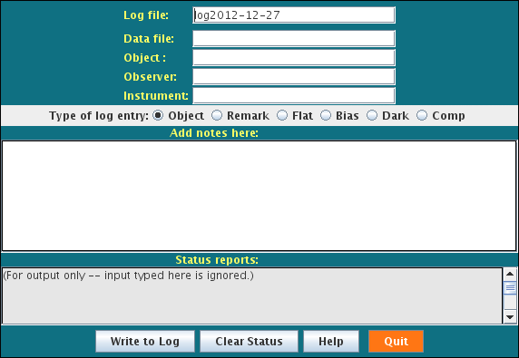
java -jar MDM13Logger.jarIt should come up with a window like this:
Every time you press the Write to Log button, the program reads the telescope and MIS information and writes it to a log file, together with the information you fill into the relevant fields. You can add whatever notes you want in the box provided -- those also get written to the log. You might want to to comment on the weather, the clock error, and so on. The Help button has more detail.
The log file is easily machine-readable, and there is a program called fillheaders.py that inserts the log file information into the headers semi-automatically. To match log entries to data files unambiguously, the best strategy is to be sure you write to the log file during the data-taking sequence. If you write the log entry before or after the sequence, fillheaders lets you match the log entry to the data more manually, but it can be a bit tedious.
Your life will be easier if you
For longer science exposures, you'll want the camera colder than for casual slit-viewing, to minimize dark current. I ran at minus-50 C during the winter, and it had no trouble holding this temperature. In cold ambient temperatures you can probably do somewhat better than this, but when it's warm your mileage may vary. I have not experimented with this. Whatever you do, it's important for the temperature to be constant -- that is, something the camera can maintain.
Notice that all the instructions for slit-viewing (above) still apply -- for setting up observations, you can use the little "RT" button to place the camera in continuous-view mode, so you can center, adjust the telescope focus, etc. Just be aware that those real-time pictures are not recorded.
(In the instructions below, recall that the tabs in Acquistion are accessed using the left-right arrows toward the upper right.)
Setup. In Acquisition, under the Setup CCD tab,
Now turn to the Binning tab. At the 1.3m, the native Andor pixels subtend 0.27 arcsec, so you probably want to make this 4x4, which gives a 128 x 128 image with 1.1 arcsec/pixel. The advantages of such severe binning are (a) smaller data sets and (b) faster read times. Simply select 4x4 binning using the radiobuttons. (It's also possible to read a sub-array, but this is not allowed for in further reductions, and the field is already small).
Now select the Auto-save tab. In here,
You should be ready to go now. To take signal, go to the Acquisition menu and simply Take Signal. The images will be displayed as they come in, and you can play with the stretch, etc., without affecting the recorded data.
During the acquisition:
Once the operation finished, you'll have a 3-dimensional FITS file in the directory you specify. The file is time-stamped to the nearest second (only), and the time between frames is given in the header to five digits or so.
For a good reduction of your data, you'll want bias, dark, and flat field exposures. Do these with exactly the same camera settings -- binning, read rate, sensor temperature, etc. -- as your science exposures. Here are some suggestions:
Between exposures (to be safe), run the Putty sftp (secure file transfer protocol) program on the windows machine. It has a little icon that looks like a terminal with a lightning bolt. It'll pop a little terminal with a command-line interface (this terminal updates oddly under VNC, but it works). I think it'll give you help if you type help, but the procedure is basically this:
If sftp doesn't work, a USB memory key works nicely, though that obviously requires physical access to the machine.
Viewing the data. As soon as you have any data to look at, use ds9 (in native mode, not IRAF!) to display the datacube:
ds9 mydata.fitsIt turns out ds9 has a wonderful and totally intuitive interface for data cubes. Photometry is a much more elaborate issue -- see the next section.
I have written a suite of python scripts to do the reductions. They use, pyraf, pyfits, and NumPy, and also my python-wrapped skycalc routines, called cooclasses. All of these are installed at MDM, but as of 2013 September, I don't have the reduction software running on the MDM workstations. I haven't had time to trace the incompatibilities yet.
Fully reducing the data involves these steps:
A disadvantage of the Andor camera is that one cannot do any photometry until the whole data cube is available, so quick-look reductions will be a little behind real time.
In these descriptions I use these rather standard notational conventions:
The reduction routines are as follows:
fillheaders.py is an elaborate program to match log entries to data files, and (in the end) to update the data file headers with the matched information. With a single file, you're asked whether to incude log entries from well before and well after the data file in question; the answer is usually no, but sometimes there will be a concluding comment or something that you typed after the integration was over, or a remark on clock error, or whatever, that would be good to include. This is a bit of a work in progress. In any case, when you've selected all your log entries, the header is updated, and comments from all the selected log entries are included.
It's important to note that flatfield data should have header information updated, because the correct filter information is needed later.
Doing photometry is slightly more elaborate. It requires the following setup files:
PIXSCALE | 1.10      # Andor 13-um pixels binned 4x4 at 1.3m f7.5
APRADIUS | 3.0       # Photometry aperture radius in arcsec.
Note the vertical bar separating the keyword from the value.
cubephot.py runs daophot aperture photometry on the images using the aperture radius from cubephot.config, and produces a data file called <image name>.ts (for "timeseries"). If the header information is installed properly, the times given are barycentric Julian dates of mid-integration minus 2450000, derived using the data cube's recorded start time, the interframe interval, the clock error, and the telescope coordinates for the barycentric correction. The next column gives the magnitude of the program object minus the magnitude of the comp star. The next is the instrumental magnitude of the comp star. Subsequent columns give instrumental magnitudes for any other stars you have measured.
Some header information (including all the comments, etc.) is given at the beginning of the file, in lines starting with "#".
The timing assumes that the cycle time that Solis writes in the headers is accurate. I have run some tests on this and the timing interval is accurate enough so that 8 hours of 10-second integrations gives a drift smaller than 3 seconds (probably quite a bit smaller).
For poorly understood reasons, the 1.3m suffers from centering drift over long exposures, even when the guider is operating. As noted earlier, the software tries to compensate for the centering drift by following the tracking star (which is usually the comp star). This can go off the rails if (e.g.) a satellite trail obliterates the tracking star in one frame. I hope to make this more robust in future versions. However, one precaution is implemented: to avoid losing track during cloudy intervals, the software stops updating the centering if the tracking star fades by 1.5 mag from its first measurement.
Once you've reduced your data and done the photometry, you'll want to look at it. I've written a little viewing program which you invoke with
viewtsphot.py [optional flags] <timeseries file name>The default values for all the flags are set for cubets.py output, so you can usually omit them.
If all goes well, it pops up a panel that looks like this:
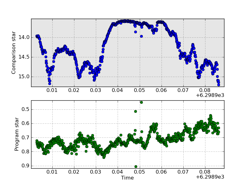
The lower panel shows the program star's differential magnitudes, the top panel shows the instrumental (non-differential) magnitude of the comparison star, and the horizontal axis is the time, by default in units of the Julian date minus 2450000. If the data have been processed with the full header information, the plotted time is barycentric (i.e. 'heliocentric'). You can see that this was a poor night -- the comp star varied by over a magnitude due to very substantial high cloud.
If you type a ? you'll get a little menu of cursor commands. Here's a summary:
Here are the optional command-line flags, some of which are not implemented. In Unix-like fashion, these are indicated with minus signs. Some have values to go with them:
In general, these options haven't been tested extensively; however, I have checked that -p <program star> will plot the differential light curve of a check star (e.g., column 3), so you can look for anything untoward.